The growth of fishes is a process through which size (weight or length) changes with time, and any attempt to depict or compare growth must deal with both of these dimensions. However, comparing growth curves, which link size and time, is not straightforward. Indeed, depending on one’s definition of ‘slow’ or ‘fast’ growth, one can get into serious contradictions when growth curves cross one another. Thus, Kinne (1960) wrote that "the difference in growth rate established in young fish does not persist throughout life. Initially slow-growing fishes may surpass initially fast-growing fishes, and finally reach a greater length-at-age." (This phenomenon is nicely illustrated in Fig. 20).
In FishBase, we use the parameters of the von Bertalanffy Growth Function or VBGF (see the ‘POPGROWTH table’, this vol.) to describe the growth of fishes. However, this does not, by itself, resolve the problem addressed by Kinne (1960), as none of these parameters has the dimensions of growth (i.e., length vs. time or weight vs. time). L
¥ and W¥ represent size alone, and K and t0 have the dimensions time-1 and time, respectively. However, various combinations of these parameters, e.g., L¥ × K have a suitable dimension (here: length× time-1), i.e., that of a growth rate (Gallucci and Quinn 1979). Put on a logarithmic basis, the indices of growth performance:Ø
’ = logK + 2logL¥ …1)and
Ø
also have the correct dimension of a growth rate, and are now widely used to compare the growth performance of different fishes and invertebrates, owing to their being normally (and narrowly) distributed for different populations of the same species (see, e.g., Moreau et al. 1986). The latter feature also allows estimation of K from L
¥ or W¥ when their (mean) Ø’ or Ø is known from a (number of) population(s) (Munro and Pauly 1983; Pauly and Munro 1984).
The slopes of 2 and 2/3 in equations (1) and (2), respectively, which make these indices perform as they do, were estimated by Pauly (1979) from a dataset documented in Pauly (1978, 1979) and now included in FishBase. Equation (1) implies that plots of logK vs. logL
¥ will have, on average, a slope of 2. Correspondingly, equation (2) implies that plots of logK vs. logW¥ will have, on average, a slope of 2/3.
An ‘auximetric’ plot (from the Greek words for ‘growth’ and ‘measure’) is a double logarithmic plot of the parameter K of the VBGF vs. asymptotic size
(L¥ or W¥ ). Herein, a population with a given set of growth parameters (L¥ , K or W¥ , K) is represented by a single point, and different populations of the same species will tend to form a cluster of points. Since equations (1) and (2) imply that these clusters can be fitted with regression lines of known slope, the clustering also implies that ellipses can be superimposed on the clusters of points, with long axes having slopes of 2, or 2/3, respectively, with intercepts equal to Ø’ or Ø, and surface areas related to the variance of the datasets that are represented.
Thus ellipses with circumference containing the 95% confidence area (S95) of a cluster of L
¥ , K (or W¥ , K) values, can be readily estimated, and a software (AUXIM), documented in Pauly et al. (1996), was developed to perform this and related functions, for files with at least 4 pairs of L¥ , K or W¥ , K values.
As AUXIM is tedious to use as a stand-alone application, a subset of its routines is included in FishBase 2000, to enable analyses of the many growth parameters therein. However, to allow comparisons among fishes of widely different shapes, only routines pertaining to growth in weight (and to
Ø, not Ø’) are included here. Also, only fishes from ‘open waters’ (and not from ‘captivity’) can be included in analyses (the reason is given in Box 16).
The auximetric analyses that can be performed within FishBase depend on one’s location in the database when invoking these analyses:
when the auximetric routines are called from within the POPULATION GROWTH INFORMATION window, all that is shown is a plot of logK vs. logW
¥
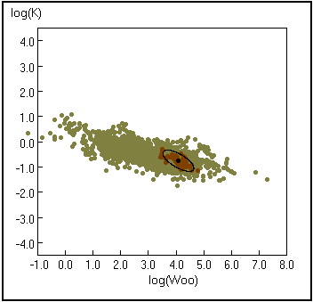
for all species in FishBase with such values (in yellow), the point(s) for the species from where the routine was invoked (in red), and an ellipse defining S95 (if the number of cases n > 4; see Box 18). Also, if n > 4, a table will be output with details on the ellipse (mean W¥
and K);
when the auximetric routines are called from the REPORTS menu, and a group of species by environment, or an order, or a family or a genus has been identified, a complete auximetric analysis can be performed, involving:
drawing of one ellipse per selected species (see Fig. 23; Box 18) and estimation of its mean K and W¥ (in cases where n < 4, the means are taken without ellipses being drawn), and display of a graph showing the ellipses and/or the means for all selected species;

Fig. 23. Plot of K vs. W¥ . Light dots represent all species for which W¥ is available in FishBase, dark dots represent entries for Gadus morhua. The ellipse with a black dot at its center represents the 95% confidence limits. See Box 18 for details.
This box, the first part of which is adapted from Pauly et al. (1996) summarizes the essential features of the approach used by AUXIM to draw ellipses. Given the VBGF weight, and the definition of Ø, we have
which is the equation of the major axis of the ellipse, with Ø as the intercept with the ordinate.
Simultaneously, and because it is perpendicular, the equation for the ellipse’s minor axis is
where Yo is the ordinate at the intercept with the ordinate axis. The abscissa of the intercept of the minor axis with the abscissa axis is
If an ellipse is to refer to the 95% confidence interval of a cloud of points, the length (2 · a) of the major axis must be related to the standard deviation of Xo°; at the same time, the length of the minor axis (2 · b) must be related to the standard deviation of Ø, or
where the value of the t-statistic is related to the number of points (n), with t = 1.96 when n = ¥
(Sokal and Rohlf 1995), and where the factor 3/2 · 3/2 · (1/ ((1 + (3/2)2)1/2) takes into account the fact that the axes of the ellipses are not parallel to the axes of the coordinate system.
When the ellipses refer to the standard deviation of the average values of logW¥
and logK, sd(Xo) and sd(Ø) are replaced by standard errors, i.e., by se(Xo) and se(Ø), respectively.
How to use AUXIM:
The user interface of AUXIM has four parts:
'Command buttons' in the upper left corner of the display with functions to: (i) increase or decrease the size of the auximetric plot (i.e., zoom-in or out); (ii) open the list of species selected prior to activating the AUXIM routine proper (available only if AUXIM was opened from the Reports Menu); and (iii) open the table of growth parameters for the current species;
Display of currently selected species and of command buttons enabling scrolling through the list (upper right corner of display);
Display tab, showing the auximetric plot, and also allowing to view the distance and overlap table, as well as the dendrogram; and
System command buttons to: (i) select or deselect a species from the list; (ii) print the current display to a printer or a file; (iii) open the help file; or (iv) close the form and return control to FishBase.
Note that functions associated with the command buttons for utilities may also be accessed by clicking the right button of the mouse. Also, the selection and deselection of species may be done through the list of species by either double-clicking on the species or by pressing the <Space Bar> to toggle the status.
Pauly, D., J. Moreau and F.C. Gayanilo, Jr. 1996. A new method for comparing the growth performance of fishes, applied to wild and farmed tilapias, p. 433-441. In R.S.V. Pullin, J. Lazard, M. Legendre, J.B. Amon Kothias and D. Pauly (eds.) The Third International Symposium on Tilapia in Aquaculture. ICLARM Conf. Proc. 41.
Sokal, R.R. and F.J. Rohlf. 1995. Biometry. Third edition. W.H. Freeman and Company, San Francisco. 887 p.
Daniel Pauly and Felimon C. Gayanilo, Jr.
estimating the distances and overlaps between species (for a minimum of 4 species), and output of these in table form; and
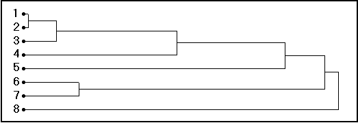
using the distances in (b) and the clustering algorithm in McCammon and Wenninger (1970) to construct a dendrogram of distances in ‘growth space’, i.e., showing the similarity of species (within the group selected) in terms of their growth (Fig. 24).

Fig. 24. Dendrogram of similarities (X-axis: arbitrary units) in ‘growth space’ as output by AUXIM for Gadidae, with 1= Theragra chalcogramma; 2 = Trisopterus luscus; 3 = Merlangius merlangus; 4 = Micromesistius poutassou; 5 = Melanogrammus aeglefinus; 6 = Gadus morhua; 7 = Pollachius virens; 8= Trisopterus minutus. As can be seen, two pairs of species (T. chalcogramma and T. luscus; G. morhua and P. virens) form the closest clusters, with subsequent clusters formed by links with other species
Analyses such as these have been performed for tilapias, Fam. Cichlidae (Pauly et al. 1996) and snappers, Fam. Lutjanidae (Pauly and Binohlan 1996), but their potential still needs to be fully explored. We are confident that such analyses will considerably expand our understanding of the growth, and generally, of the biology of fishes, and we look forward to users’ feedback on this.
An auximetric graph¾ albeit without elipse¾ can be created by clicking on the Auximetric graph link in the list of growth parameters for a given species, which is created by clicking on the Growth link in the ‘More information’ section of the ‘Species Summary’ page.
Gallucci, V.F. and T.J. Quinn, II. 1979. Reparameterizing, fitting, and testing a simple growth model. Trans. Am. Fish. Soc. 108(1):14-25.
Kinne, O. 1960. Growth, food intake, and food consumption in an europlastic fish exposed to different temperatures and salinities. Physiol. Zool. 33:288-317.
McCammon, R.B. and G. Wenninger. 1970. The dendrograph. Computer Contribution 48. State Geological Survey. The University of Kansas, Lawrence. 26 p.
Moreau, J., C. Bambino and D. Pauly. 1986. A comparison of four indices of overall fish growth performance, based on 100 tilapia populations (Fam. Cichlidae), p. 201-206. In J.L. Maclean, L.B. Dizon and L.V. Hosillos (eds.) The First Asian Fisheries Forum. Asian Fisheries Society, Manila, Philippines.
Munro, J.L. and D. Pauly. 1983. A simple method for comparing the growth of fishes and invertebrates. Fishbyte 1(1):5-6.
Pauly, D. 1978. A preliminary compilation of fish length growth parameters. Ber. Inst. Meereskd. Christian-Albrechts Univ. Kiel 55, 200 p.
Pauly, D. 1979. Gill size and temperature as governing factors in fish growth: a generalization of von Bertalanffy’s growth formula. Ber. Inst. Meereskd. Christian-Albrechts Univ. Kiel 63, 156 p.
Pauly, D. and J.L. Munro. 1984. Once more on the comparison of growth in fish and invertebrates. Fishbyte 2(1):21.
Pauly, D. and C. Binohlan. 1996. FishBase and AUXIM as tools for comparing the life-history patterns, growth and natural mortality of fish: applications to snappers and groupers, p. 223-247. In F. Arreguin-Sánchez, J.L. Munro, M.C. Balgos and D. Pauly (eds.) Biology, fisheries and culture of tropical groupers and snappers. ICLARM Conf. Proc. 48.
Pauly, D., J. Moreau and F.C. Gayanilo, Jr. 1996. A new method for comparing the growth performance of fishes, applied to wild and farmed tilapias, p. 433-441. In R.S.V. Pullin, J. Lazard, M. Legendre, J.B. Amon-Kothias and D. Pauly (eds.) The Third International Symposium on Tilapia in Aquaculture. ICLARM Conf. Proc. 41.
Daniel Pauly, Jacques Moreau and Felimon C. Gayanilo, Jr.